Display3D: a stream mechanism for displaying 3D DGtal objects

Table of Contents

• Display3D: a stream mechanism from abstract class Display3D
• Interactive visualization from Viewer3D
• Static visualization from Board2Dto3D
• Visualization of DigitalSet and digital objects
• Mode selection: the example of digital objects in 3D
• Useful modes for several 3D drawable elements
  • Listing of different modes
  • Examples with Objet modes
  • Illustrating KhalimskyCell with the "Illustration" mode
• Changing the style for displaying drawable elements.
• Adding clipping planes

This part of the manual describes how to visualize 3D objects and how to import them from binary file (.obj or pgm3d)

Author:

Bertrand Kerautret, Martial Tola

Display3D: a stream mechanism from abstract class Display3D

The semi abstract class Display3D defines the stream mechanism to display 3d primitive (like PointVector, DigitalSetBySTLSet, Object ...). The class Viewer3D and Board3DTo2D implement two different ways to display 3D objects. The first one (Viewer3D), permits an interactive visualisation (based on OpenGL) and the second one (Board3DTo2D) provides 3D visualisation from 2D vectorial display (based on the CAIRO library).

Interactive visualization from Viewer3D

The class Viewer3D inherits from the base class QGLViewer (which is based on QGLwidget). It permits to display simple 3D shapes. LibQGLViewer ( http://www.libqglviewer.com ) is a C++ library based on QT allowing to access to simple 3D fonctionalities like camera moving, mouse, keyboard interaction, clipping plane .... etc.

First to use the Viewer3D stream, you need to include the following hearders:

 #include "DGtal/io/3dViewers/Viewer3D.h"

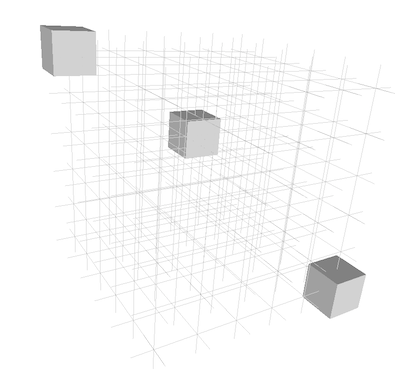
The following code snippet defines three points and a rectangular domain in Z3. It then displays them in a Viewer3D object. The full code is in viewer3D-1-points.cpp.

The first step to visualize 3D object with Viewer3D is to create a QApplication from the main():

using namespace DGtal;
using namespace Z3i;

QApplication application(argc,argv);
Viewer3D viewer;
viewer.show();

Then we can display some 3D primitives:

 Point p1( 0, 0, 0 );
 Point p2( 5, 5 ,5 );
 Point p3( 2, 3, 4 );
 Domain domain( p1, p2 );

 viewer << domain;  
 viewer << p1 << p2 << p3; 
 viewer << Viewer3D::updateDisplay;

You should obtain the following visualisation:

Digital point visualization with Viewer3D.

Note:

Note that you can display the camera settings in the console (key C) which can be used in Board2Dto3D described in the following.

Static visualization from Board2Dto3D

The same visualization can be obtain with the Board2Dto3D class. You just need to adapt the camera settings (see example: dgtalBoard3DTo2D-1-points.cpp ).

Board3DTo2D viewer;
viewer << domain;  
viewer << p1 << p2 << p3;
  
viewer << CameraPosition(2.500000, 2.500000, 16.078199)
       << CameraDirection(0.000000, 0.000000, -1.000000)
       << CameraUpVector(0.000000, 1.000000, 0.000000);
viewer << CameraZNearFar(4.578200, 22.578199);
viewer.saveCairo("dgtalCairo-1-points.pdf", Board3DTo2D::CairoPDF, 600*2, 400*2);

This example should provides a comparable visualization.

Visualization of DigitalSet and digital objects

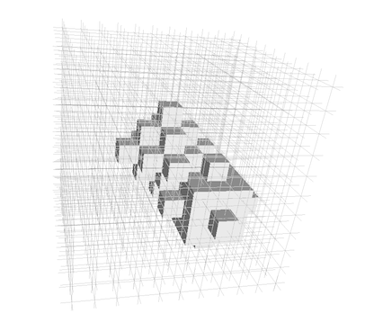
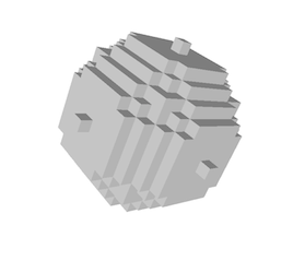
The Viewer3D class allows also to display directly a DigitalSet. The first step is to create a DigitalSet for example from the Shape class.

 QApplication application(argc,argv);
 Viewer3D viewer;
 viewer.show();

 Point p1( 0, 0, 0 );
 Point p2( 10, 10 , 10 );
 Domain domain( p1, p2 );
 viewer << domain;
 
 DigitalSet shape_set( domain );
 Shapes<Domain>::addNorm1Ball( shape_set, Point( 5, 5, 5 ), 2 );
 Shapes<Domain>::addNorm2Ball( shape_set, Point( 3, 3, 3 ), 2 );
 
 shape_set.erase(Point(3,3,3));
 shape_set.erase(Point(6,6,6));
 viewer << shape_set << Viewer3D::updateDisplay

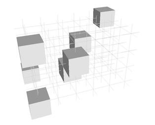
You should obtain the following visualisation (see example: viewer3D-2-sets.cpp ):

Digital point visualization with Viewer3D.

Mode selection: the example of digital objects in 3D

As for Board2D, a mode can be choosed to display elements (SetMode3D). You just have to specify the classname (the easiest way is to call the method className() on an instance of the correct type and the desired mode (a string).

 Object6_18 shape( dt6_18, shape_set );
 viewer << SetMode3D( shape.className(), "DrawAdjacencies" );
 viewer << shape;

*or change the couple of adjacency

 Object18_6 shape2( dt18_6, shape_set );
 viewer << SetMode3D( shape2.className(), "DrawAdjacencies" );
 viewer << shape2;

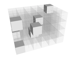
You should obtain the two following visualisations (see example: viewer3D-3-objects.cpp ):

6-18 digital Adjacencies visualization with Viewer3D.

18-6 digital Adjacencies visualization with Viewer3D.

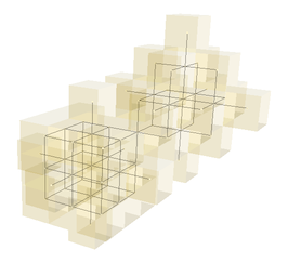
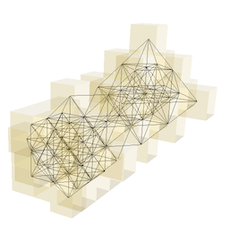
Note that digital set was displayed with transparency by setting a custom colors.

Useful modes for several 3D drawable elements

Listing of different modes

As for Board2D the object can be displayed with different possible mode:

• class PointVector, modes: "" / "Both", "Paving" (default), "Grid"
• class DigitalSetBySTLSet and DigitalSetBySTLVector : "", "" / "Both", "Paving" (default), "PavingTransp", "Grid".
• class Object, modes: "" /"Basic" (default), "DrawAdjacencies", "PavingTransp".
• class HyperRectDomain, modes: "" / "Grid" (default), "Paving", "PavingPoints", "PavingGrids", "BoundingBox".
• class KhalimskyCell , modes: ""(default) / "Highlighted" , "Transparent", "Basic", "Illustration", "IllustrationCustomColor".
• class SignedKhalimskyCell , modes: "" (default) / "Highlighted" , "Basic", "Transparent", "Illustration", "IllustrationCustomColor".

Note that for KhalimskyCell and SignedKhalimskyCell the defaul colors (with CustomColors3D objects) can be changed only with the empty mode ("") and "IllustrationCustomColor" mode.

Examples with Objet modes

The file viewer3D-4-modes.cpp illustrates several possible modes to display these objects:

We can display the set of point and the domain

 Point p1( -1, -1, -2 );
 Point p2( 2, 2, 3 );
 Domain domain( p1, p2 );
 Point p3( 1, 1, 1 );
 Point p4( 2, -1, 3 );
 Point p5( -1, 2, 3 );
 Point p6( 0, 0, 0 );
 Point p0( 0, 2, 1 );

without mode change (see image (a)):

 viewer << p1 << p2 << p3<< p4<< p5 << p6 << p0;
 viewer << domain;

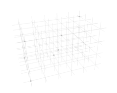
We can change the mode for displaying the domain (see image (b)):

 viewer << p1 << p2 << p3<< p4<< p5 << p6 << p0;
 viewer << SetMode3D(domain.className(), "PavingGrids");
 viewer << domain;

(Note that to avoid transparency displaying artifacts, we need to display the domain after the voxel elements included in the domain)

It is also possible to change the mode for displaying the voxels: (see image (c))

viewer << domain;
viewer <<  SetMode3D( p1.className(), "Grid" );
viewer << p1 << p2 << p3<< p4<< p5 << p6 << p0;

we obtain the following visualisations:

(a) Default visualisation of a digital point sets with the associated domain

(b) Visualisation using Paving mode for the domain.

(c) Visualisation using Paving mode for the voxels.

Illustrating KhalimskyCell with the "Illustration" mode

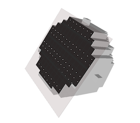
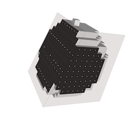
The "Illustration" mode is defined to construct illustrations composed of KhalimskyCell. In particular it permits to increase the space between cells and improve the display visibility. It can be used typically as follows: First you need to add the following header:

#include "DGtal/io/DrawWithDisplay3DModifier.h"

From a SignedKhalimskyCell (SCell in DGtal::Z3i) you have to select the "Illustration" mode :

  SCell v = K.sSpel( Point( 0, 0, 0 ), KSpace::POS ); // +v
  viewer << SetMode3D( v.className(), "Illustration" );

Then, to display a surfel with its associated voxel, you need to transform the surfel by constructing a shifted and resized version (DGtal::TransformedKSSurfel) according to its associated voxel:

  SCell sx = K.sIncident( v, 0, true ); // surfel further along x  
  DGtal::TransformedKSSurfel tsx (sx, v);

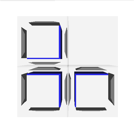
You will obtain such type of illustration (obtained from the example viewer3D-4bis-illustrationMode.cpp ).

Illustration of the "Illustration" KhalimskyCell mode.

Changing the style for displaying drawable elements.

As for Board2D, it is possible to custom the way to display 3D elements by using an instance of the following classes:

• CustomColors3D: to change the color used to display surface primitive (GL_QUADS) and the pen color (LINE/POINTS) ;

The custom color can be applied by an instance of the CustomColors3D as follow:

  viewer << CustomColors3D(Color(250, 0,0),Color(250, 0,0));
  viewer << p4 << p5 ;

The example viewer3D-5-custom.cpp illustrates some possible customs :

Example of several custom display .

Adding clipping planes

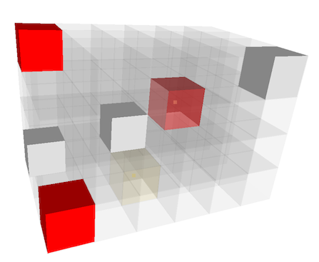
It also possible through the stream mechanism to add clipping plane with the object ClippingPlane. We just have to add the real plane equation and adding as for displaying an element. The file viewer3D-6-clipping.cpp gives a simple example.

From displaying a digital set defined from a Norm2 ball,

 Point p1( 0, 0, 0 );
 Point p2( 20, 20, 20 );
 Domain domain(p1, p2);
 DigitalSet shape_set( domain );

 Shapes<Domain>::addNorm2Ball( shape_set, Point( 10, 10, 10 ), 7 );

 viewer << SetMode3D( shape_set.className(), "Both" );
 viewer << shape_set;
 viewer << CustomColors3D(Color(250, 200,0, 100),Color(250, 200,0, 20));
 viewer <<  SetMode3D( p1.className(), "Paving" );

we can add for instance two differents clipping planes:

 viewer << ClippingPlane(1,0,0,-4.9);
 viewer << ClippingPlane(0,1,0.3,-10);

(a) Visualisation of the initial set.

(b) Visualisation after adding the first clipping plane (0,1,0.3,-10).

(c) Visualisation after adding a second clipping plane (1,0,0,-4.9) .