This work is part of the project

The quality provided by image/video sensors increases steadily, and for a fixed spatial resolution the sensor noise has been gradually reduced. However, modern sensors are also capable of acquiring at higher spatial resolutions which are still affected by noise, specially at low lighting conditions. The situation is even worse in video cameras, where the capture time is bounded by the frame rate. The noise in the video degrades its visual quality and hinders its analysis.
We propose a new patch-based video denoising method based on an empirical Bayesian approach. The method assumes that the noise is white, additive and Gaussian and that each spatio-temporal 3D patch in the unknown clean sequence is a sample drawn from an a priori Gaussian distribution. This distribution can be learnt using the most similar noisy patches, and then the clean patch can be estimated by computing the maximum a posteriori. The method does rely on an acurate motion estimation, and compares favourably to state-of-the-art methods in color and grayscale classic test sequences.
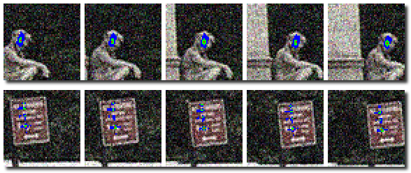
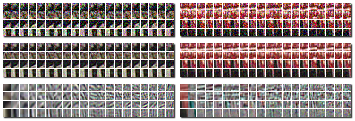
Fig. 1 shows two examples of groups of 200 similar 3D patches used to learn the a priori Gaussian distribution. Fig. 2 shows the noisy patches in the group, the corresponding MAP estimates of the clean patches and the mean and principal directions of the learnt Gaussian model. The final denoised video is given by the aggretation of these MAP estimates.
P. Arias, J.-M. Morel, Towards a Bayesian Video Denoising Method,
Proc. Advanced Concepts for Intelligent Vision Systems,
2015, pg. 107-117.
P. Arias, J.-M. Morel, Video denoising via empirical Bayesian estimation of space-time patches,
preprint, 2017.
In Table 1, we show results obtained for five classic color test sequences,
with the proposed method, in its variant VNLB-S, using patches of size 10x10x2.
The sequence names in the table header and some of the PSNR values in the table
are links to the corresponding videos. The videos are uncompressed.
We compared our results with:
V-BM3D: [Dabov, Foi, Egiazarian. 2007]
V-BM4D-tip: [Maggioni et al. 2012]
V-BM4D-mp: author's implementation of
[Maggioni et al. 2012]
setting the parameters according to the modified profile (best parameter profile available)
| σ | Method | Tennis | Coastguard | Foreman | Bus | Football | Average |
|---|---|---|---|---|---|---|---|
| 10 | Noisy | 28.13 | 28.13 | 28.13 | 28.13 | 28.13 | |
| V-BM3D | 36.04 | 36.82 | 37.52 | 34.96 | 36.34 | ||
| V-BM4D-tip | 36.42 | 37.27 | 37.92 | 36.23 | 36.96 | ||
| V-BM4D-mp | 35.90 | 36.30 | 37.21 | 35.38 | 36.08 | 36.20 | |
| VNLB-S | 36.88 | 38.01 | 39.05 | 37.94 | 37.62 | 37.97 | |
| 20 | Noisy | 22.11 | 22.11 | 22.11 | 22.11 | 22.11 | |
| V-BM3D | 32.54 | 33.39 | 34.49 | 31.03 | 32.86 | ||
| V-BM4D-tip | 32.88 | 33.61 | 34.62 | 32.27 | 33.35 | ||
| V-BM4D-mp | 31.98 | 32.44 | 33.70 | 31.34 | 32.22 | 32.37 | |
| VNLB-S | 33.35 | 34.50 | 35.78 | 34.42 | 33.99 | 34.51 | |
| 40 | Noisy | 16.09 | 16.09 | 16.09 | 16.09 | 16.09 | |
| V-BM3D | 29.20 | 29.99 | 31.17 | 27.34 | 29.43 | ||
| V-BM4D-tip | 29.52 | 30.00 | 31.30 | 28.32 | 29.78 | ||
| V-BM4D-mp | 28.14 | 28.73 | 30.09 | 27.44 | 28.35 | 28.60 | |
| VNLB-S | 29.92 | 31.19 | 32.60 | 30.69 | 30.36 | 31.10 | |
In Table 2, we show results obtained for five classic grayscale test sequences,
with the two variants of the proposed method, VNLB-H and VNLB-S, using patches of size 10x10x2.
The sequence names in the table header and some of the PSNR values in the table
are links to the corresponding videos. The videos are uncompressed.
We compared our results with:
V-BM4D-tip: [Maggioni et al. 2012]
V-BM4D-mp: author's implementation of
[Maggioni et al. 2012]
setting the parameters according to the modified profile (best parameter profile available)
| σ | Method | Tennis | Salesman | Fl. garden | Mobile | Bicycle | Stefan | Average | ||||||
|---|---|---|---|---|---|---|---|---|---|---|---|---|---|---|
| 10 | Noisy | 28.13 | 28.13 | 28.13 | 28.13 | 28.13 | 28.13 | |||||||
| V-BM4D-tip | 35.22 | 37.30 | 32.81 | 37.66 | ||||||||||
| V-BM4D-mp | 34.95 | 37.48 | 32.01 | 34.11 | 37.85 | 33.68 | 35.01 | |||||||
| VNLB-S | 35.89 | 38.36 | 34.42 | 36.37 | 39.37 | 35.83 | 36.71 | |||||||
| VNLB-H | 36.00 | 38.62 | 34.61 | 36.67 | 39.53 | 36.02 | 36.91 | |||||||
| 20 | Noisy | 22.11 | 22.11 | 22.11 | 22.11 | 22.11 | 22.11 | |||||||
| V-BM4D-tip | 31.59 | 33.79 | 28.63 | 34.10 | ||||||||||
| V-BM4D-mp | 31.08 | 33.46 | 28.32 | 30.49 | 34.54 | 29.69 | 31.26 | |||||||
| VNLB-S | 32.14 | 34.73 | 30.24 | 32.42 | 36.22 | 31.70 | 32.91 | |||||||
| VNLB-H | 32.20 | 34.99 | 30.46 | 32.82 | 36.45 | 31.94 | 33.14 | |||||||
| 40 | Noisy | 16.09 | 16.09 | 16.09 | 16.09 | 16.09 | 16.09 | |||||||
| V-BM4D-tip | 28.49 | 30.35 | 24.60 | 30.10 | ||||||||||
| V-BM4D-mp | 28.38 | 29.37 | 24.59 | 26.02 | 30.58 | 25.64 | 27.43 | |||||||
| VNLB-S | 29.14 | 30.89 | 26.18 | 28.24 | 32.44 | 27.71 | 29.10 | |||||||
| VNLB-H | 29.24 | 31.09 | 26.29 | 28.55 | 32.70 | 27.84 | 29.29 | |||||||