The influence of exterior unknown values on interior image values
Abstract.
The goal of these notes is to provide a theoretical framework to evaluate the precision of image values inside the image domain, taking into account that by Shannon theory, these values for a band limited image depend on the exterior, unknown values. Since the exterior values are actually unknown the evaluation of this precision requires a model. Following other studies [] and in particular Shannon’s proposal, we take as worst case the case where the image inside and outside is a white noise. This permits easy theoretical computations and actually corresponds to a worst case but also to a realistic case. This is realistic because real digital images have noise and contain microtexture whose characteristics is close to white noise. This is a worst case because digital images have a decay spectrum that is significantly faster than the white noise spectrum (which is flat). Therefore among band-limited digital images white noise has the least predictable samples from neighborhoods. The calculations deliver quantitative security rules. They give us a guaranteed image accuracy depending on the distance from the image boundary, and show that for large images the inside values actually depend marginally on the outside values, up to a narrow security band on the boundary.
1 The error caused by the ignorance of outside samples
1.1 The case of 1D signals
We shall start the calculations in 1D.
We denote the sinus cardinal function ![]() Its Fourier transform is supported in
Its Fourier transform is supported in ![]() . In such a case we shall say that the function is “band limited”. The system
. In such a case we shall say that the function is “band limited”. The system ![]() ,
, ![]() is an orthonormal system of the set of band limited functions in
is an orthonormal system of the set of band limited functions in ![]() . By Shannon-Whittaker theorem, a function
. By Shannon-Whittaker theorem, a function ![]() is band limited if and only if the sequence
is band limited if and only if the sequence ![]() belongs to
belongs to ![]() and
and
| (1) |
Our general model for an unknown function will be a stationary white noise. This noise will represent the unknown samples, being outside the signal domain. Consider a noise ![]() whose samples are
whose samples are ![]() independent real variables. The sum
independent real variables. The sum ![]() is almost surely unbounded. Nevertheless we can still use the Shannon-Whittaker formula (1). Indeed
set
is almost surely unbounded. Nevertheless we can still use the Shannon-Whittaker formula (1). Indeed
set ![]() Then
Then
 |
This series is uniformly bounded with respect to ![]() . By Lebesgue theorem it follows that the function
. By Lebesgue theorem it follows that the function ![]() belongs to
belongs to ![]() almost surely and that the above series converges in
almost surely and that the above series converges in ![]() . Thus we can make a sense of the Shannon-Whittaker
. Thus we can make a sense of the Shannon-Whittaker ![]() interpolate of a white uniform noise, defined as the limit in
interpolate of a white uniform noise, defined as the limit in ![]() as
as ![]() of the Shannon-Whittaker interpolate of a the truncated noise
of the Shannon-Whittaker interpolate of a the truncated noise ![]() . Thus, even if in practice we end up playing with finitely many samples, it is convenient to consider this white noise interpolate.
. Thus, even if in practice we end up playing with finitely many samples, it is convenient to consider this white noise interpolate.
We assume that the ![]() are the samples of a band limited function in
are the samples of a band limited function in ![]() . The samples
. The samples ![]() are known for
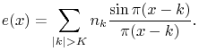
are known for ![]() and the rest is unknown and can have arbitrary values that we model in a worst case strategy by a white noise
and the rest is unknown and can have arbitrary values that we model in a worst case strategy by a white noise ![]() . Here we shall consider several “extrapolation” possibilities that will turn out equivalent for the error analysis (I am not yet sure that this statement is really true).
There are actually two classical extrapolation for the missing samples (we could think of the DCT as well - it assumes a mirror symmetry before periodizing). The first is to decide that the samples
. Here we shall consider several “extrapolation” possibilities that will turn out equivalent for the error analysis (I am not yet sure that this statement is really true).
There are actually two classical extrapolation for the missing samples (we could think of the DCT as well - it assumes a mirror symmetry before periodizing). The first is to decide that the samples ![]() outside the observed domain
outside the observed domain ![]() are null. Then the Shannon-Wittaker interpolation will be faulty, and the error
are null. Then the Shannon-Wittaker interpolation will be faulty, and the error ![]() between the original and the interpolated one will be
between the original and the interpolated one will be ![]() . The alternative consists in a periodization of the observed image. It corresponds to the use of the discrete Fourier transform to interpolate the known samples
. The alternative consists in a periodization of the observed image. It corresponds to the use of the discrete Fourier transform to interpolate the known samples ![]() amounts to assuming that the outside samples are mere repetitions of
amounts to assuming that the outside samples are mere repetitions of ![]() . This discrete case will differ a little and we shall consider it later on.
Now we focus on the error analysis caused by the ignorance of the samples
. This discrete case will differ a little and we shall consider it later on.
Now we focus on the error analysis caused by the ignorance of the samples ![]() ,
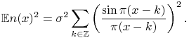
, ![]() . We have just seen that the error caused inside the domain, namely for
. We have just seen that the error caused inside the domain, namely for ![]() , satisfies
, satisfies
 |
(2) |
Thus the error variance is
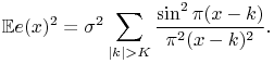 |
(3) |
For ![]() in the signal domain
in the signal domain ![]() , define the distances to the (respectively left and right) boundary
, define the distances to the (respectively left and right) boundary ![]() . We shall estimate how
. We shall estimate how ![]() varies as a function of these distances. Starting with
varies as a function of these distances. Starting with ![]() , we obtain
, we obtain
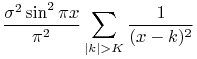 |
||||
 |
||||
Note, the third line (i.e. the first inequality) is obtained by using an argument of decreasing function. Wa can use the same argument but to get a lower bound of the error and then obtain the following feasible range
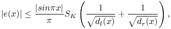
We have proved
Lemma 1.
The error ![]() on the value at
on the value at ![]() of a band limited function whose samples are known on an interval
of a band limited function whose samples are known on an interval ![]() and whose unknown samples are i.i.d. with variance
and whose unknown samples are i.i.d. with variance ![]() outside the domain satisfies
outside the domain satisfies
where ![]() and
and ![]() are the integer parts of the distances of
are the integer parts of the distances of ![]() to the left/right boundaries.
to the left/right boundaries.
Besides, the tightness of this upper bound can be estimated as
1.2 Extension to 2D images
We now proceed to the 2D extension of the above estimate. The 2D model is
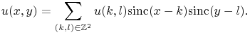 |
(4) |
The error formula becomes
![\mathbb{E}e(x,y)^{2}=\sigma^{2}\sum _{{(k,l)\in\mathbb{Z}^{2}\setminus[-K,K]^{2}}}\frac{\sin^{2}\pi(x-k)}{\pi^{2}(x-k)^{2}}\frac{\sin^{2}\pi(y-l)}{\pi^{2}(y-l)^{2}}.](mi/mi31.png) |
(5) |
Using the respective horizontal and vertical distances ![]() and
and ![]() of
of ![]() to the boundary of the square
to the boundary of the square ![]() , assuming without loss of generality that
, assuming without loss of generality that ![]() , and using11The mentioned formula is a straightforward consequence of the Shannnon-Whittaker interpolation formula with
, and using11The mentioned formula is a straightforward consequence of the Shannnon-Whittaker interpolation formula with ![]() at
at ![]() the identity
the identity ![]() , we obtain
, we obtain
 |
||||
 |
||||
Theorem 1.
The expected square error ![]() on the value at
on the value at ![]() of a band limited image whose samples are known on a domain
of a band limited image whose samples are known on a domain ![]() and whose unknown samples are i.i.d. with variance
and whose unknown samples are i.i.d. with variance ![]() outside this domain satisfies
outside this domain satisfies
where ![]() and
and ![]() (resp.
(resp. ![]() and
and ![]() ) are the integer parts of the distances of
) are the integer parts of the distances of ![]() (resp.
(resp. ![]() ) to the left/right (resp. lower/upper) boundaries.
) to the left/right (resp. lower/upper) boundaries.
In short denoting by ![]() the taxi driver distance of
the taxi driver distance of ![]() to the image boundary, and having
to the image boundary, and having ![]() while
while ![]() remains bounded, the error bound behaves like
remains bounded, the error bound behaves like ![]()
1.3 Discussion
We can first give some orders of magnitude. A typical digital image has standard deviation of about ![]() . Thus avoiding an error
. Thus avoiding an error ![]() larger than
larger than ![]() , requires by the preceding result
, requires by the preceding result ![]() . Since digital images nowadays are very large, this estimate is somewhat reassuring. Indeed, an order 1 error on colors escapes our attention and the security zone to remove is small if not negligible for images that attain respectable widths of
. Since digital images nowadays are very large, this estimate is somewhat reassuring. Indeed, an order 1 error on colors escapes our attention and the security zone to remove is small if not negligible for images that attain respectable widths of ![]() pixels and more. On the other hand, this estimate clearly hinders using cameras as high precision numerical tools. Furthermore, the error caused by our ignorance of the image outside its domain remains serious even far inside the image domain, since it decreases like the square root of the distance to the boundary.
pixels and more. On the other hand, this estimate clearly hinders using cameras as high precision numerical tools. Furthermore, the error caused by our ignorance of the image outside its domain remains serious even far inside the image domain, since it decreases like the square root of the distance to the boundary.
Besides, the problem of the truncation error bound has been studied in previous literature, in the case of deterministic signals. It is interesting to note that form of the error estimate presented in Lemma 1 bears a strong resemblance with the ones in [5, 3]. Note that [2] has also studied similar bounds but for a slightly different interpolation, and we will not study the comparison in this case. However, a more careful comparison with these two works reveals subtle distinctions. First of all, both bounds are obtained under deterministic model.
The closest formula is this proposed in [3], which under our notations becomes:
 |
where ![]() . Note that for a white noise
. Note that for a white noise ![]() is almost-surely unbounded.
is almost-surely unbounded.
In [5], the formula is a bit different:
where, ![]() and
and ![]() is the upper bound of the frequencies present in
is the upper bound of the frequencies present in ![]() .
.
Note also that many articles (at least [5, 2]) impose a frequency guard band regarding the strict Nyquist limit.
2 The error caused by missing outside samples for DFT interpolation
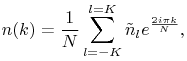
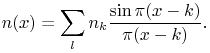
Again we start studying the phenomenon in 1D. Now we consider the classic DFT interpolation. This interpolation starts with the samples ![]() . Computing the discrete Fourier transform of this vector yields
. Computing the discrete Fourier transform of this vector yields ![]() Fourier coefficients,
Fourier coefficients,
 |
(6) |
obtained from the samples ![]() ,
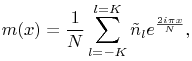
, ![]() , which can themselves be recovered by the discrete inverse Fourier transform
, which can themselves be recovered by the discrete inverse Fourier transform
 |
(7) |
where for a sake of concision we set ![]() .
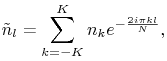
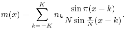
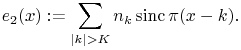
In this framework the function
.
In this framework the function ![]() is implicitly assumed to be
is implicitly assumed to be ![]() periodic, which is of course simply not true. Indeed, its DFT interpolate is the Fourier truncated series
periodic, which is of course simply not true. Indeed, its DFT interpolate is the Fourier truncated series
 |
(8) |
where ![]() is clearly distinct from
is clearly distinct from ![]() . Thus our goal is to evaluate the difference between
. Thus our goal is to evaluate the difference between ![]() and the lawful Shannon-Whittaker interpolate (assuming all samples known),
and the lawful Shannon-Whittaker interpolate (assuming all samples known),
 |
(9) |
To evaluate ![]() our first goal will be to put (8) in a form similar to (9). To do so we can substitute (6) in (7),
our first goal will be to put (8) in a form similar to (9). To do so we can substitute (6) in (7),
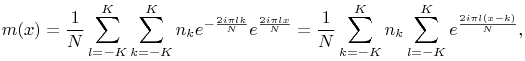 |
which after some reorganization yields the classic DFT interpolation formula
 |
(10) |
By subtracting (10) from (9) we obtain a closed formula for the error
![]() with
with
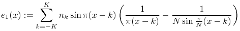 |
and
 |
We have already evaluated ![]() in the preceding section. Thus we have to evaluate
in the preceding section. Thus we have to evaluate ![]() .
In the following we normalize the space variable
.
In the following we normalize the space variable ![]() so that when
so that when ![]() , the signal domain becomes
, the signal domain becomes ![]() .
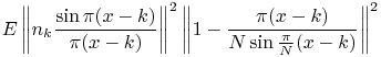
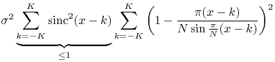
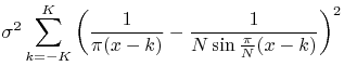
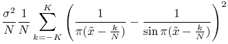
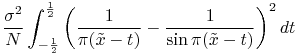
By the Riemann sum theorem we have
.
By the Riemann sum theorem we have
![\displaystyle\mathbb{E}\left[\sum _{{k=-K}}^{K}n_{k}\sin\pi(x-k)\left(\frac{1}{\pi(x-k)}-\frac{1}{N\sin\frac{\pi}{N}(x-k)}\right)\right]^{2}](mi/mi25.png) |
(11) | ||||
![\displaystyle\mathbb{E}\left[\sum _{{k=-K}}^{K}n_{k}\left(\frac{\sin\pi(x-k)}{\pi(x-k)}\right)\left(1-\frac{\pi(x-k)}{N\sin\frac{\pi}{N}(x-k)}\right)\right]^{2}](mi/mi24.png) |
(12) | ||||
 |
(13) | ||||
 |
(14) | ||||
| (15) |
 |
(16) | ||||
 |
(17) | ||||
 |
(18) | ||||
 |
(19) |
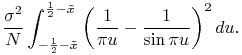
This means that no matter where ![]() is in the signal domain, the error between Shannon and DFT is
is in the signal domain, the error between Shannon and DFT is ![]() . We now pass to estimate how the error grows near the domain boundary. Thus we assume that
. We now pass to estimate how the error grows near the domain boundary. Thus we assume that ![]() . Then the above integral is
. Then the above integral is ![]() . Indeed, the singluarities present in the integral at its upper bound (which tends to
. Indeed, the singluarities present in the integral at its upper bound (which tends to ![]() ) cancel out. And the singular term introduced when the lower bound tends to
) cancel out. And the singular term introduced when the lower bound tends to ![]() is
is ![]() In other term using that
In other term using that ![]() , the term bounding
, the term bounding ![]() is equivalent to
is equivalent to ![]() , which means that the term bounding
, which means that the term bounding ![]() depends on the distance of
depends on the distance of ![]() to the domain boundary and is of order
to the domain boundary and is of order ![]()
Although this equivalent is correct, the above estimates need some refinement. First we need to replace the inequality in (11) by a real equivalent. Second, we have made above two successive equivalence arguments which need some more rigor. The solution to avoid the inequality is to replace the upper bound on ![]() by an equality, which can be probably done by using Cauchy Schwartz before taking the expectation of the square of
by an equality, which can be probably done by using Cauchy Schwartz before taking the expectation of the square of ![]() . The chain of equivalences can be straightened by replacing them by asymptotic expansions.
. The chain of equivalences can be straightened by replacing them by asymptotic expansions.
2.1 test
References
-
A sampling theorem for duration-limited functions with error estimates,Information and Control 34 (1), pp. 55–65.External Links: Link.Cited by: 1.3.
-
Sampling theorem for the fourier transform of a distribution with bounded support,SIAM Journal on Applied Mathematics 16 (3), pp. 626–636.
-
Bounds for truncation error of the sampling expansion,SIAM Journal on Applied Mathematics 14 (4), pp. 714–723.
-
On the approximation by truncated sampling series expansions,Signal processing 7 (2), pp. 191–197.Cited by: 1.3.
-
On truncation error bounds for sampling representations of band-limited signals,Aerospace and Electronic Systems, IEEE Transactions on (6), pp. 640–647.