Author:: David Coeurjolly

This part of the manual describes the DGtal volumetric package and its classes. We focus here on separable process based volumetric analysis such as distance transformation, reverse distance transformation and medial axis extraction.

Introduction

For decades, distance transformation (DT) and geometrical skeleton extraction have been classic tools for shape analysis [ROSEN_66,ROSEN_68]. The DT of a shape consists in labelling object grid points with the distance to the closest background pixel. From the DT values, we thus have information on the shape geometry. Beside its applications in shape description, DT has been used in many situations such as shape analysis, shape matching, shape-based interpolation, motion planning, image registration, or differential measurement estimation.

In the literature, many techniques have been proposed to compute the DT given a metric with a trade-off between algorithmic performances and the accuracy of the metric compared to the Euclidean one. Hence, many papers have considered distances based on chamfer masks [ROSEN_68,BORGE_86], or sequences of chamfer distances; the vector displacement based Euclidean distance [DANI_80,RAGN_90,MULL_92] the Voronoi diagram based Euclidean distance [BREU_95, MAUR_2003] or the square of the Euclidean distance [SAITO_94,HIRA_96]. From a computational point of view, several of these methods lead to time optimal algorithms to compute the error-free Euclidean Distance Transformation (EDT) for n- dimensional binary images: the extension of these algorithms is straightforward since they use separable techniques to compute the DT; n one-dimensional operations -one per direction of the coordinate axis- are performed.

In [COEU_07], it has been demonstrated that a similar decomposition can be used to compute both the reverse distance transformation and a discrete medial axis of the binary shape.

In fact, the separable decomposition and the associated algorithmic tools can be used on a wider class of metrics (see [HIRA_96] or [MAUR_2003]). For instance, all weighted $l_p$ metrics defined in $R^n$ by

\[ d_{L_p} (u,v) = \left ( \sum_{i=0}^n w_i|u_i-v_i |^p \right )^{\frac{1}{p}}\]

can be considered.

In DGtal, we have chosen to separate the metric from the algorithmic details. We discuss in section Separable Metric Traits on the construction of a separable metric type.

Distance Transformation

Given a binary object $ X $ and its complementary $\bar{X}$, the distance transformation is a mapping of points $ x\in X$ with distance values such that

\[ DT(x) = \min_{y\in\bar{X}} ( d(x,y)) \]

For the Euclidean metric in dimension 2, it is equivalent to

\[ DT(x) =\sqrt{ \min_{y\in\bar{X}} ( (x_0-y_0)^2 + (x_1-y_1)^2 ) } \]

with $x(x_0,x_1)\in R^2$.

Hence, the key point for exact computations is to consider square of distances and to represent these quantities as integers. In other words, we have to specify a type for the output values such that it can be used to represent square of input integers (to be precise, n sums of squares in dimension n). For $l_p$ metrics, the output type should be able to represent integers made of sums of numbers $ (x_i-y_i)^p$.

As a consequence, the class DistanceTransformation is parametrized by three elements:

a type representing the underlying digital space (model of CSpace);
a type representing the object $ X $ as a point predicate (model of CPointPredicate) ;
and a static number "p" used to define the $l_p$ metric.

An optional fourth IntegerLong template parameter with default type DGtal::int64_t can be specified to represent the sums of $x_i^p$ values. This type is important because it corresponds to the Value type of the DistanceTransformation::OutputImage type that is used to store the output result.

Hence, the DistanceTransformation class provides

a output image type;
a method to compute the distance transformation of an input image.

Note:: The output image type provided by DistanceTransformation is a ImageContainerBySTLVector whose domain specification is copied from the input image type and whose value type is IntegerLong to return exact values.

The class constructor has got two arguments:

a domain on which the computation is done;
an instance of the point predicate.

Warning:: The point predicate must be defined (i.e. must return true or false) for each point of the input domain.

For example (using the DGtal::StdDefs shortcuts), let us consider the following input:

  Z2i::Point a ( 0, 0 );
  Z2i::Point b ( 127, 127);
  
  //Input image with unsigned char values
  typedef ImageSelector<Z2i::Domain, unsigned int>::Type Image;
  Image image ( Z2i::Domain(a, b ));
  //We fill the image with the 128 value
  for ( Image::Iterator it = image.begin(), itend = image.end();it != itend; ++it)
    (*it)=128;
  //We generate 16 seeds with 0 values.
  randomSeeds(image,16,0);

In this example, the image is filled with 128 values and 16 random sites are set to 0 (function randomSeeds).

From this image, we need to construct a point predicate which will return true for 128 values and false otherwise. Hence, we use a simple threshold:

  //Point Predicate from random seed image
  typedef SimpleThresholdForegroundPredicate<Image> PointPredicate;
  PointPredicate predicate(image,0);

Now, the following code computes the distance transformation on this image for the $l_1$, $l_2$ and $l_\infty$ metrics (see distancetransform2D.cpp for a complete example) .

  typedef  DistanceTransformation<Z2i::Space, PointPredicate, 2> DTL2;
  typedef  DistanceTransformation<Z2i::Space, PointPredicate, 0> DTLInf;
  typedef  DistanceTransformation<Z2i::Space, PointPredicate, 1> DTL1;
 
 
  DTL2 dtL2( image.domain(), predicate );
  DTLInf dtLinf(image.domain(), predicate );
  DTL1 dtL1(image.domain(),  predicate );
  
  DTL2::OutputImage resultL2 = dtL2.compute (  );
  DTLInf::OutputImage resultLinf = dtLinf.compute (  );
  DTL1::OutputImage resultL1 = dtL1.compute (  );

Few comments can be made from this example. First, Z2i::Image is defined on a Z2i::Domain whose pixel coordinates Z2i::Space::Coordinate have type DGtal::int32_t. In this example, we have used the default DGtal::uint64_t type to store sum of two square of Coordinate differences. Since the capacity of the output image value type is important for memory issues, the method DistanceTransformation::checkTypesValidity can check at runtime the type validity (based on the image size and dimension to have a tighter estimation).

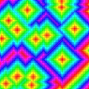
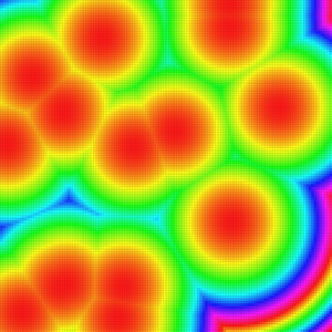
Here you have the resulting distance images using appropriate colormaps (note that for the l_2 metric, the square of the distance values are mapped).

l_1 distance transformation in 2D

l_2 distance transformation in 2D

l_infty distance transformation in 2D

If you want to characterize $ X $ as a digital set, here you have an example of the predicate construction:

Z2i::Domain domain(Z2i::Point(-10,-10), Z2i::Point(10,10));
Z2i::DigitalSet aSet(domain);
aSet.insertNew(Point(2,2));
//... more point insertions
//Predicate construction
typedef DGtal::SetPredicate<Z2i::DigitalSet> Predicate;
Predicate aPredicate(aSet);
//DT computation (euclidean metric)
DGtal::DistanceTransformtion<Z2i::Space, Predicate, 2> dt(domain,aPredicate);
DGtal::DistanceTransformtion<Z2i::Space, Predicate, 2>::OutputImage out = dt.compute();

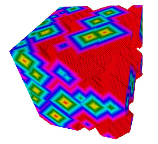
A simple example applying the 3D transform (see distancetransform3D.cpp). This program outputs these images (L1 metric):

l_1 distance transformation in 3D

Reverse Distance Transformation

Given a set of balls and a domain, the aim of the reverse reconstruction is to compute the binary shape defined as the union of the input balls. In other word, a point x belong to the set $X$ is there exists at least one ball containing $x$.

This notion is deeply linked to the distance transformation computation since it can interpreted as a reverse operator:

\[ REDT(DT(X)) = X \]

In DGtal, the input set of balls is specified by an image and a grid point with value greater than 0 indicates a ball. Hence, the ReverseDistanceTransformation class has a similar usage than the DistanceTransformation one:

Z2i::Point a ( 0, 0 );
Z2i::Point b ( 127, 127);
//Input image with unsigned char values
typedef ImageSelector<Z2i::Domain, unsigned int>::Type Image;
Image image ( a, b );
//...
// set values in image (by default 0-value pixels are background
// pixels, otherwise, see ForegroundPredicate in DistanceTransformation).
//...
// Point predicate construction
typedef SimpleThresholdForegroundPredicate<Image> PointPredicate;
PointPredicate predicate(image,0);
 
//Definition of the DistanceTransformation operator for the l_2 metric
typedef DistanceTransformation< Z2i::Space, Predicate, 2> DTL2;
typedef DTL2::OutputImage OutputImage
DTL2 dt(Domain(a,b), predicate);
OutputImage result = dt.compute(  );
//Definition of the ReverseDistanceTransformation opertor for the l_2
//metric
typedef ReverseDistanceTransformation< OutputImage, 2> RDTL2;
typedef RDTL2::OutputImage OutputReconstruction;
RDTL2 rdt;
OutputReconstruction reconstruction = rdt.reconstruction(results);
//we can check that reconstruction ~ image

From this example, we can notice that: the first template parameter type of ReverseDistanceTransformation is an image type whose Value must be consistent with the $l_p$ metric as discussed in the DistanceTransformation section; the second parmeter is the static integer $p$.

There is an optional third template parameter to specify the value type of the output binary image (default is DGta::int8_t). During the construction of the rdt object, we can also optionnaly specify the value used to represent object grid points (set $X$, default value is 1) and background grid points (default value is '0'). For instance

RDTL2 rdt(128,0);

will affect the value 128 to object points and 0 otherwise.

Warning:: Obviously, the reconstruction will be incorrect if the metric used in the distance transformation is not the same as the metric used for the reconstruction.

Discrete Medial Axis Extraction

Todo:: complete code/doc

Separable Metric Traits

As discussed in the introduction, the same algorithmic decomposition can be used on different metrics. In DGtal, such suitable metrics are models of the concept CSeparableMetric, defined in the SeparableMetricTraits class. At this point, we have specialization for the Euclidean metric ( $l_2$), the Chessboard distance ( $l_1$) and the Manhattan distance

Warning:: In SeparableMetricTraits the power "p" is a static number of type DGtal::uint32_t. Hence, to specify a $l_\infty$ metric, we use the value "0" for the template parameter "p" (and thus we forbid the use of $l_0$ metric). It does not make sense in a mathematical point of view but it makes the code simpler.

References

G. Borgefors. Distance transformations in digital images. Computer Vision, Graphics, and Image Processing, 34(3):344–371, June 1986.

D. Coeurjolly and A. Montanvert. Optimal separable algorithms to compute the reverse euclidean distance transformation and discrete medial axis in arbitrary dimension. IEEE Transactions on Pattern Analysis and Machine Intelligence, 29(3):437–448, March 2007.

P.-E. Danielsson. Euclidean distance mapping. Computer Graphics and Image Processing, 14:227–248, 1980.

T. Hirata. A unified linear-time algorithm for computing distance maps. Information Processing Letters, 58(3):129–133, May 1996.

C.R.Maurer,R.Qi,andV.Raghavan.A linear time algorithm for computing exact euclidean distance transforms of binary images in arbitrary dimensions. IEEE Transactions on Pattern Analysis and Machine Intelligence, 25(2):265–270, February 2003.

J.C. Mullikin. The vector distance transform in two and three dimensions. Computer Vision, Graphics, and Image Processing. Graphical Models and Image Processing, 54(6):526–535, November 1992.

I. Ragnemalm. Contour processing distance transforms, pages 204–211. World Scientific, 1990.

A. Rosenfeld and J. L. Pfaltz. Sequential operations in digital picture processing. Journal of the ACM, 13(4):471–494, October 1966.

A. Rosenfeld and J. L. Pfalz. Distance functions on digital pictures. Pattern Recognition, 1:33–61, 1968.

T. Saito and J I Toriwaki. New algorithms for Euclidean distance transformations of an $n$- dimensional digitized picture with applications. Pattern Recognition, 27:1551–1565, 1994.