|
DGtal
0.6.devel
|


All Data Structures Namespaces Files Functions Variables Typedefs Enumerations Enumerator Friends Groups Pages
|
DGtal
0.6.devel
|
This part of the manual describes how to extract patterns from one-dimensional discrete structures (basically digital curves).
The goal is to provide tools that help in analysing any one-dimensional discrete structures in a generic framework. These structures are assumed to be constant, not mutable. This is a (not exhaustive) list of such structures used in digital geometry:
Since these structures are one-dimensional and discrete, they can be viewed as a locally ordered set of elements, like a string of pearls. Two notions are thus important: the one of element and the one of local order, which means that all the elements (except maybe at the ends) have a previous and next element. The concept of iterator is heavily used in our framework because it encompasses these two notions at the same time: like a pointer, it provides a way of moving along the structure (operator++, operator–) and provides a way of getting the elements (operator*).
In the following, iterators are assumed to be constant (because the structures are assumed to be constant) and to be at least bidirectionnal (ie. they are either bidirectionnal iterators or random access iterators). You can read the STL documentation about iterators: http://www.sgi.com/tech/stl/Iterators.html to learn more about the different kind of iterators.
The notion of reachability is very important. An iterator j is reachable from an iterator i if and only if i can be made equal to j with finitely many applications of the operator++. If j is reachable from i, one can iterate over the range of elements bounded by i and j, from the one pointed to by i and up to but not including the one pointed to by j. Such a range is valid and is denoted by [i,j).
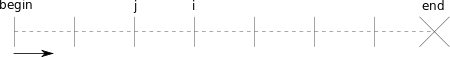
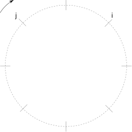
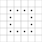
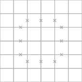
Let i and j be two iterators that point to two elements of a same structure. For open (or linear) structures, [i,j) is not always a valid range (ie. j is not always reachable from i) because if j has not been reached and if i points to the last element, one application of the operator++ makes i to be equal to the past-the-end value, ie. an iterator value that points past the last element (just as a regular pointer to an array guarantees that there is a pointer value pointing past the last element of the array). If i turns out to be equal to the past-the-end value, then j cannot be reached from i. If an iterator denoted by begin points to the first element of a given structure and an iterator denoted by end is the past-the-end value, iterating over the range [begin,end) is a way of iterating over all the elements of the underlying structure. If the underlying structure is empty, it only has a past-the-end value. As a consequence, a range [i, i) denotes an empty range. A range of a linear structure is illustrated below (normal values are depicted with a small straight segment, whereas the past-the-end value is depicted with a cross). In this example, [i,j) is not a valid range because j cannot be reached from i and the whole range may be denoted by [begin,end).
@subsection geometryGridCurve GridCurve and FreemanChain.
Two objects are provided in DGtal to deal with digital curves: GridCurve and FreemanChain.
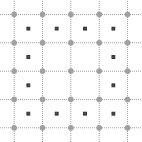
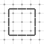
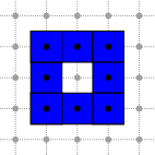
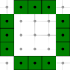
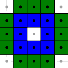
GridCurve is an (open or closed) n-dimensional oriented grid curve. It stores a list of alternated (signed) 0-cells and 1-cells, but provides many ranges to iterate over different kinds of elements:
You can get an access to these nine ranges through the following methods:
The different ranges for a grid curve whose chain code is 1110002223333 are depicted below.
As GridCurve, it provides a CodesRange.
Each range has the following inner types:
And each range provides these (circular)iterator services:
You can use these services to iterate over the elements of a given range as follows:
Since GridCurve and FreemanChain have both a method isClosed(), you can decide to use a classic iterator or a circulator at running time as follows:
In this section, we focus on parts of one-dimensional structures, called segment. More precisely, a segment is a valid and not empty range. Any model of the concept CSegment, should have the following inner types:
and the following methods:
Moreover, a segment can be defined from a property P, which can be built from conjunctions and disjunctions of other properties. A given property P is valid iff it is true for any valid range of only one element and true for any valid range of any segment for which P is true. For instance, the properties "to be a 4-connected DSS" or "to be a balanced word" can define segments, but "to contain at least k elements (k > 1)" cannot define segments because it does not hold for ranges of strictly less than k elements.
In digital geometry, a primitive is usually defined as a class of digital objects: the Gauss digitization of a Euclidean disk is an example of primitive. In this framework, a primitive is the class of segments verifying the same valid property P.
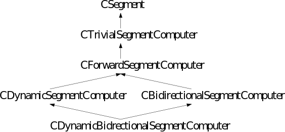
The detection problem consists in deciding whether a given segment belongs to a class of segments defined from a valid property P or not. If P is valid, the detection of a segment can be performed in an incremental way: a segment is initialized at a starting element and then can be extended to the neighbors elements if the property P still holds. A segment that can control its own extension (so that P remains true) is a segment computer. A segment computer is not a single concept, but actually five concepts that form a hierarchy: the first one can only extend itself in one direction, while others define additional functionality. The five concepts that are actually used in segmentation algorithms are CTrivialSegmentComputer, CForwardSegmentComputer, CBidirectionalSegmentComputer, CDynamicSegmentComputer and CDynamicBidirectionalSegmentComputer.
Detecting a segment in a range looks like this:
If the underlying structure is closed, infinite loops are avoided as follows:
Segment computers are based on iterators. This is a useful feature since it provides a way to iterate over the segment if it is required at some points of the detection process. However the extension of a segment can be performed in only one direction (given by operator++). To cope with this problem, the models of CForwardSegmentComputer, which is a refinement of CTrivialSegmentComputer, should define the following nested type:
Reverse is a type that behaves like Self but with reverse iterators. Moreover, in order to build an instance of Self (resp. Reverse) from a segment computer, the following method should be defined:
The returned objects may not be full copies of this, may not have the same internal state as this, but must be constructed from the same input parameters so that they can detect segments verifying the same property. For instance, in digital geometry, k-arcs detection may be implemented as a segment computer constructed from the input parameter k indicating the adjacency to use. In this case, getSelf and getReverse methods must return segment computers based on the k-adjacency too. These segment computers may be not valid before calling the init method.
As the name suggests, forward segment computers can only extend themselves in the forward direction, but this direction is relative to the direction of the underlying iterators (the direction given by operator++ for instances of Self, but the direction given by operator– for instances of Reverse) They cannot extend themselves in two directions at the same time around an element contrary to bidirectional segment computers.
Any model of CBidirectionalSegmentComputer, which is a refinement of CForwardSegmentComputer, should define the following methods:
GeometricalDSS and GeometricalDCA are both models of CBidirectionalSegmentComputer.
The concept CDynamicSegmentComputer is another refinement of CForwardSegmentComputer. Any model of this concept should define the following method:
Finally, the concept CDynamicBidirectionalSegmentComputer is a refinement of both CBidirectionalSegmentComputer and CDynamicSegmentComputer and the define this extra method:
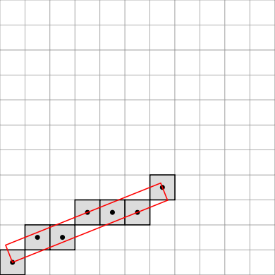
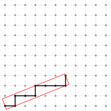
A model of CDynamicBidirectionalSegmentComputer is the class ArithmeticalDSS, devoted to the dynamic recognition of DSSs, defined as a sequence of connected points \( (x,y) \) such that \( \mu \leq ax - by < \mu + \omega \) (see Debled and Reveilles, 1995).
Here is a short example of how to use this class in the 4-connected case:
Here is a short example of how to use this class in the 8-connected case:
These snippets are drawn from ArithmeticalDSS.cpp.
The resulting DSSs of the two previous pieces of code are drawing below:
See Board2D: a stream mechanism for displaying 2D digital objects for the drawing mechanism.
As seen above, the code can be different if an iterator or a circulator is used as the nested ConstIterator type. Moreover, some tasks can be made faster for a given kind of segment computer than for another kind of segment computer. That's why many generic functions are provided in SegmentComputerUtils.h:
These functions are used in the segmentation algorithms introduced below.
A given range contains a finite set of segments verifying a given valid property P. A segmentation is a subset of the whole set of segments, such that:
i. each element of the range belongs to a segment of the subset and
ii. no segment contains another segment of the subset.
Due to (ii), the segments of a segmentation can be ordered without ambiguity (according to the position of their first element for instance).
Segmentation algorithms should verify the concept CSegmentation. A CSegmentation model should define the following nested type:
It should also define a constructor taking as input parameters:
Note that a model of CSegmentComputerIterator should define the following methods :
@subsection geometryGreedyDecomposition Greedy segmentation
The first and simplest segmentation is the greedy one: from a starting element, extend a segment while it is possible, get the last element of the resulting segment and iterate. This segmentation algorithm is implemented in the class GreedySegmentation.
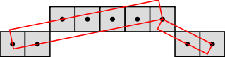
 In the short example below, a digital curve stored in a STL vector
 is decomposed into 8-connected DSSs whose parameters are sent to
 the standard output.
 @code
//types definition typedef PointVector<2,int> Point; typedef std::vector<Point> Range; typedef Range::const_iterator ConstIterator; typedef ArithmeticalDSS<ConstIterator,int,8> SegmentComputer; typedef GreedySegmentation<SegmentComputer> Segmentation;
//input points Range curve; curve.push_back(Point(1,1)); curve.push_back(Point(2,1)); curve.push_back(Point(3,2)); curve.push_back(Point(4,2)); curve.push_back(Point(5,2)); curve.push_back(Point(6,2)); curve.push_back(Point(7,2)); curve.push_back(Point(8,1)); curve.push_back(Point(9,1));
//Segmentation SegmentComputer recognitionAlgorithm; Segmentation theSegmentation(curve.begin(), curve.end(), recognitionAlgorithm);
Segmentation::SegmentComputerIterator i = theSegmentation.begin(); Segmentation::SegmentComputerIterator end = theSegmentation.end(); for ( ; i != end; ++i) { SegmentComputer current(*i); trace.info() << current << std::endl; //standard output }
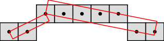
If you want to get the DSSs segmentation of the digital curve when it is scanned in the reverse way, you can use the reverse iterator of the STL vector:
The resulting segmentations are shown in the figures below:
If you want to get the DSSs segmentation of a part of the
digital curve (not the whole digital curve), you can give
the range to process as a pair of iterators when calling
the setSubRange() method as follow:
@code
theSegmentation.setSubRange(beginIt, endIt);
Obviously, [beginIt, endIt) has to be a valid range included in the wider range [curve.begin(), curve.end()).
Moreover, a part of a digital curve may be processed either as an independant (open) digital curve or as a part whose segmentation at the ends depends of the underlying digital curve. That's why 3 processing modes are available:
In order to set a mode (before getting a SegmentComputerIterator), use the setMode() method as follow:
Note that the default mode will be used for any unknown modes.
The complexity of the greedy segmentation algorithm relies on the complexity of the extendForward() method of the segment computer. If it runs in (possibly amortized) constant time, then the complexity of the segmentation is linear in the length of the range.
A unique and richer segmentation, called saturated segmentation, is the whole set of maximal segments (a maximal segment is a segment that cannot be contained in a greater segment). This segmentation algorithm is implemented in the class SaturatedSegmentation.
In the previous segmentation code, instead of the line:
it is enough to write the following line:
to get the following figure:
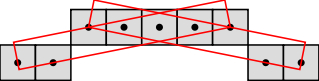
See convex-and-concave-parts.cpp for an example of how to use maximal DSSs to decompose a digital curve into convex and concave parts.
If you want to get the saturated segmentation of a part of the digital curve (not the whole digital curve), you can give the range to process as a pair of iterators when calling the setSubRange() method as follow:
Obviously, [beginIt, endIt) has to be a valid range included in the wider range [curve.begin(), curve.end()).
Moreover, the segmentation at the ends depends of the underlying digital curve. Among the whole set of maximal segments that pass through the first (resp. last) element of the range, one maximal segment must be chosen as the first (resp. last) retrieved maximal segments. Several processing modes are therefore available:
The mode i indicates that the segmentation begins with the i-th maximal segment passing through the first element and ends with the i maximal segment passing through the last element.
In order to set a mode (before getting a SegmentComputerIterator), use the setMode() method as follow:
Note that the default mode will be used for any unknown modes.
The complexity of the saturated segmentation algorithm relies on the complexity of the functions available for computing maximal segments (firstMaximalSegment, lastMaximalSegment, mostCenteredMaximalSegment, previousMaximalSegment and nextMaximalSegment), which are specialized according to the type of segment computer (forward, bidirectional and dynamic).
Let \( l \) be the length of the range and \( n \) the number of maximal segments. Let \( L_i \) be the length of the i-th maximal segments. During the segmentation, the current segment is extended:
Moreover, note that \( \Sigma_{1 \leq i \leq n} L_i \) may be equal to \( O(l) \) (for instance for DSSs).
 1.8.1.1