- Author(s) of this documentation:
- Jacques-Olivier Lachaud
Part of the Geometry package.
This module gathers classes and functions to recognize piece of naive planes, and more generally piece of planes with arbitrary rational axis-thickness. It is based on an implementation of the COBA Algorithm [Charrier, Buzer 1998 : Charrier:2008-dgci]. For the user, everything is gathered in classes COBANaivePlane and COBAGenericNaivePlane, which are additive primitive computers. File viewer3D-7-planes.cpp gives a very simple example of use-case. File greedy-plane-segmentation.cpp is a non trivial example that uses this plane recognition algorithm.
Related examples are viewer3D-7-planes.cpp, greedy-plane-segmentation.cpp, greedy-plane-segmentation-ex2.cpp.
What planes are recognized by the COBA algorithm ?
The COBA algorithm recognizes planes defined with some equation \( \mu \le \vec{N} \cdot \vec{x} < \mu + \epsilon \), where \( N_z \) (for instance) is 1. This is ok for instance for recognizing naive planes defined by \( d \le ax+by+cz < d + \omega \) where \( \omega = \max(a,b,c) \). Assign indeed \( \mu = d / \omega, \vec{N} = (a,b,c) / \omega, \epsilon = 1 \). Extension to integer multiples or rational multiples of such planes is straightforward, and is hence provided.
The user thus specifies a main axis axis and a rational width (i.e. \( \epsilon \) as widthNumerator / widthDenominator ) at initialization (see COBANaivePlane::init()).
The idea of the COBA algorithm is to transform the problem into a linear integer programming problem in the digital plane \( Z^2 \). If the main axis is z, then the algorithm looks for unknown variables \( (N_x,N_y) \). Given a set of points \( (\vec{P}_i) \), it computes (or maintains in the incremental form) the 2D space of solutions induced by these points. More precisely, each point induces two linear constraints \( \mu \le \vec{N} \cdot \vec{P}_i \) and \( \vec{N} \cdot \vec{P}_i < \mu + \epsilon \).
Instead of keeping this problem in \( R^2 \), the problem is cast in \( (hZ)^2 \), where the parameter h is the sampling step and is sufficiently small to capture a solution when there is one. When initializing the algorithm, the user must give the diameter of the set of points \( (\vec{P}_i) \) (here largest vector in \(\infty\) norm), see COBANaivePlane::init().
It is proven that if \( 0 < h < 1/(2D^3) \), where D is the diameter, then if there is a solution, there is a rational solution with denominator less than \( 2D^3 \).
The COBA algorithm uses therefore a 2D lattice polytope (a convex polygon with vertices at integer coordinates), and class LatticePolytope2D, to maintain the set of rational solutions. Experimentally, even for a great number of points (<=100000), this convex set has generally fewer than 12 vertices (see Extracting plane characteristics).
A drawback of the COBA algorithm is that it does not provide the minimal characteristics of the recognized plane. This is due to the sampling method. In practice, the extracted normal is close to the minimal (integer) one.
- Note:
- Another problem is that parameter \( \mu \) is also unknown. To cope with that problem, a given solution (the centroid) is picked up and the maximal and minimal bounds are computed from it. If for a new point the bounds are too big, then a new direction is chosen by following the gradient of the induced constraints, and the algorithm optimizes iteratively the direction so as to get a direction with feasible bounds or no solutions. All this is hidden to the user, but explains the worst-case complexity.
-
You may have a look at Arithmetic package, more precisely at module Lattice polytopes in the digital plane ZxZ (convex polygons with vertices at integer coordinates) to see how lattice polytopes are represented.
How to recognize a plane ?
The main class is COBANaivePlane. It is templated by the digital space TSpace, an arbitrary model of CSpace with dimension equal to 3, and by the internal integer type TInternalInteger, which should be an integral type with big enough precision to perform computations in the subsampled \( Z^2 \).
The most important inner types are (most of the others are redefinitions so that this object is a model of boost::ForwardContainer):
- Point: the type of point that will be checked in the algorithm. Defined as TSpace::Point.
- InternalInteger: the type of integer used in computations. Defined as TInternalInteger.
- PointSet: the type that defines the set of points stored in this object (for now, std::set<Point>).
- ConstIterator: the type of iterator to visit the set of points that composed the currently recognized plane.
You may instantiate a COBANaivePlane as follows:
#include "DGtal/arithmetic/COBANaivePlane.h"
...
using namespace Z3i;
...
plane.init( 2, 100, 1, 1 );
Assuming you have a sequence of points stored in a container v, you may recognize if it is a piece of z-axis naive plane with the following piece of code:
bool isZNaivePlane( const vector<Point> & v )
{
COBANaivePlane<Z3, int64_t> plane;
plane.init( 2, 500, 1, 1 );
for ( vector<Point>::const_iterator it = v.begin(), itEnd = v.end();
it != itEnd; ++it )
if ( ! plane.extend( *it ) ) return false;
return true;
}
Therefore, the main methods for recognizing a plane are:
- COBANaivePlane::extend(const Point &): given a Point, it updates this plane such that it includes also this new point. If this is possible, it returns
true, otherwise it returns false and the object is in the same state as before the call.
- COBANaivePlane::isExtendable(const Point &)const: given a Point, it checks whether or not there is a plane that includes also this new point. It returns
true in this case, otherwise it returns false. The object is left unchanged whatever the result.
- Note:
- Calling COBANaivePlane::isExtendable before COBANaivePlane::extend does not induce a speed up on the second method. You should prefer calling directly COBANaivePlane::extend() whenever you wish to extend the plane at this point.
You may also have a look at example viewer3D-7-planes.cpp.
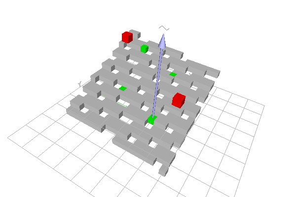
Piece of naive plane containing the four green points. There is no naive plane containing also any one of the red points.
- Note:
- TInternalInteger specifies the type of integer used in internal computations. The type should be able to hold integers of order (2*D^3)^2 if D is the diameter of the set of digital points. In practice, diameter is limited to 20 for int32_t, diameter is approximately 500 for int64_t, and whatever with BigInteger/GMP integers. For huge diameters, the slow-down is polylogarithmic with the diameter.
Extracting plane characteristics
You may obtain the current normal to the plane as a 3D vector over some real-value type (e.g. float, double) with the templated methods COBANaivePlane::getNormal (one component has norm 1) and COBANaivePlane::getUnitNormal (the 2-norm of the vector is 1).
You may obtain the upper and lower bounds of the scalar products with COBANaivePlane::getBounds.
- Note:
- The COBA algorithm does not give you the minimal characteristics of the plane that contains all the input points. It provides you one feasible solution.
Speed and computational complexity of COBA algorithm
It is not a trivial task to determine bounds on the computational complexity of this algorithm that depends only on the number of points N. Indeed, the determinant factor on the complexity is the number of times k that the plane parameters are updated. Another factor is the number of vertices v of the current convex set of solutions.
- The parameter k depends on the order of added point. It is related to the depth of bidimensional continued fraction of the plane normal (since each update corresponds to a refinement of the plane normal). A rule of thumb upper bound is some \( O(\log^2(D)) \), but experiments suggest a much lower bound.
- The parameter v seems mostly bounded in experiments. It is of course bounded by \( O(D^\frac{2}{3}) \), which is the 2D lattice polytope with the maximum number of sides in a D x D box. However, experiments suggest a more likely \( \log \log D \).
- Note also that each time a new point is inserted, we check if it has already been added. With std::set, this implies a \(O(\log N)\) cost.
Putting everything together gives some \( O(N \log N + k(v+N+\log(D))\log^2(D)) \). Neglecting v gives \( O( N (\log N + k \log^3 D ) ) \).
We have runned the following benchmark to estimate the average speed of COBA algorithm. For each experiment, 1000 naive planes were randomly chosen. Then, for an input diameter D, N points are randomly chosen in the parallelepiped D x D x D, such that they belong to the plane. We measure the time T to recognize these points as a naive plane (all calls to extend succeed). We also measure the number of updates k for this recognition. The following figures show the obtained results for a number of points varying from 50 to 100000 and a diameter varying from 50 to 1000000. It shows that the algorithm performs better in practice than the given upper bounds, even assuming \( k = \log \log D \) and v constant.
- Note:
- All computations were made with TInternalInteger set to BigInteger.
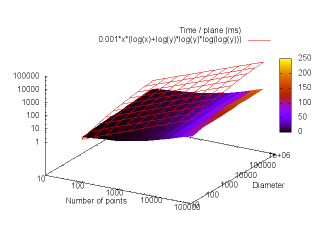
Time (in ms) to recognize a naive plane as a function of the number of points N (x-axis) and the diameter (y-axis). Time is averaged over 1000 random recognitions.
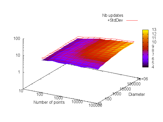
Number of updates (and deviation) when recognizing a naive plane, as a function of the number of points N (x-axis) and the diameter (y-axis). This number is averaged over 1000 random recognitions.
Application to greedy segmentation into digital planes
Example greedy-plane-segmentation.cpp illustrates the use of COBANaivePlane to segment a digital surface into connected pieces of digital planes.
The surface will be define as some digital surface in a thresholded 3D image. The image is loaded here.
QApplication application(argc,argv);
typedef ImageSelector < Domain, int>::Type Image;
SetFromImage<DigitalSet>::append<Image>(set3d, image, threshold,255);
Then the digital surface is built within this volume.
KSpace ks;
bool ok = ks.init( set3d.domain().lowerBound(),
set3d.domain().upperBound(), true );
if ( ! ok ) std::cerr << "[KSpace.init] Failed." << std::endl;
SurfelAdjacency<KSpace::dimension> surfAdj( true );
MyDigitalSurfaceContainer* ptrSurfContainer =
new MyDigitalSurfaceContainer( ks, set3d, surfAdj );
MyDigitalSurface digSurf( ptrSurfContainer );
We define a few types. Note the COBANaivePlane and the structure SegmentedPlane, which will store information for each plane.
using namespace Z3i;
typedef DigitalSetBoundary<KSpace,DigitalSet> MyDigitalSurfaceContainer;
typedef DigitalSurface<MyDigitalSurfaceContainer> MyDigitalSurface;
typedef SurfelSet::iterator SurfelSetIterator;
typedef BreadthFirstVisitor<MyDigitalSurface>
Visitor;
Color color;
};
We proceed to the segmentation itself. Note that we iterate over each surface element (surfel or vertex). Only vertices not processed can define the starting point of a new plane. Then a breadth-first traversal is initiated from this vertex and vertices are added to the plane as long as it is possible.
std::set<Vertex> processedVertices;
std::vector<SegmentedPlane*> segmentedPlanes;
std::map<Vertex,SegmentedPlane*> v2plane;
Point p;
unsigned int j = 0;
unsigned int nb = digSurf.size();
for ( ConstIterator it = digSurf.begin(), itE= digSurf.end(); it != itE; ++it )
{
Vertex v = *it;
if ( processedVertices.find( v ) != processedVertices.end() )
continue;
segmentedPlanes.push_back( ptrSegment );
axis = ks.sOrthDir( v );
ptrSegment->
plane.
init( axis, 500, widthNum, widthDen );
while ( ! visitor.finished() )
{
v = node.first;
if ( processedVertices.find( v ) == processedVertices.end() )
{
axis = ks.sOrthDir( v );
p = ks.sCoords( ks.sDirectIncident( v, axis ) );
if ( isExtended )
{
processedVertices.insert( v );
v2plane[ v ] = ptrSegment;
visitor.expand();
}
else
visitor.ignore();
}
else
visitor.ignore();
}
ptrSegment->
color = Color( random() % 256, random() % 256, random() % 256, 255 );
}
We display it using 3D viewers.
Viewer3D viewer;
viewer.show();
for ( std::map<Vertex,SegmentedPlane*>::const_iterator
it = v2plane.begin(), itE = v2plane.end();
it != itE; ++it )
{
viewer << CustomColors3D( it->second->color, it->second->color );
viewer << ks.unsigns( it->first );
}
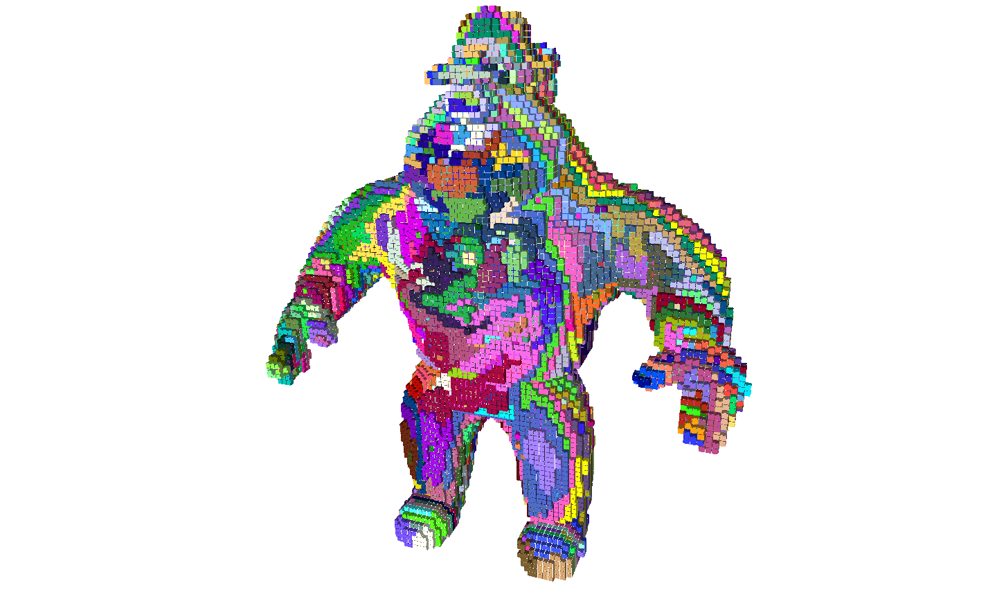
Greedy segmentation of Al capone into naive planes.
- Note:
- This approach to plane segmentation is very naive. Because there are favored axes when iterating (vertices are not randomly picked up), this technique has indeed the drawback of favoring "slice planes", which are not very useful.
-
Exercice 1. Randomize the greedy plane recognition. The simplest approach is first to put all vertices into a vector, then suffle it with STL algorithms. And then iterate over this shuffled set.
-
Exercice 2. Enhance the polyhedrization by selecting first the vertices that induces the biggest planes. This is much slower than above, but will give nicer results. For each vertex, computes its best plane by breadth-first traversal. Stores the obtained size (or better moments). Do that for each vertex independently. Put them in a priority queue, the first to be popped should be the ones with the biggest size. The remaining of the algorithm is unchanged.
What if you do not know the main axis beforehands ?
In this case, you should use the class COBAGenericNaivePlane. You use it similarly to COBANaivePlane, but you do not need to specify a main axis when calling COBAGenericNaivePlane::init().
#include "DGtal/arithmetic/COBAGenericNaivePlane.h"
...
using namespace Z3i;
...
plane.init( 100, 1, 1 );
Then, you may use methods COBAGenericNaivePlane::clear(), COBAGenericNaivePlane::extend(), COBAGenericNaivePlane::isExtendable(), etc, similarly as for class COBANaivePlane. The advantage is that the object detects progressively what is the correct main axis. You may know what is a correct main axis by calling COBAGenericNaivePlane::active().
- Note:
- The principle of COBAGenericNaivePlane is to have three instances of COBANaivePlane at the beginning, one per possible axis. When extending the object by adding points, all active instances are extended. If any one of the active instance fails, it is removed from the active instances. It is guaranteed that if there is a naive plane (of specified width) that contains the given set of points, then the object COBAGenericNaivePlane will have at least one active COBANaivePlane instance. COBAGenericNaivePlane is thus a correct recognizer of arbitrary pieces of naive planes.


 1.8.1.1